DFS & BFS
DFS:Depth First Search,深度优先搜索算法,是一种以stack实现的算法。
BFS:Breath First Search,广度优先搜索算法,是一种以queue实现的算法。
stack和queue的区别:stack是先进后出,queue是先进先出。
假设我们已知一个graph如下:
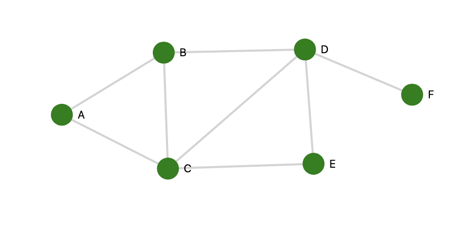
首先我们使用DFS来遍历整个图
我们需要把图的数据录入到
dict里面1
2
3
4
5
6
7
8graphs = {
'A': ['B', 'C'],
'B': ['A', 'C', 'D'],
'C': ['A', 'B', 'D', 'E'],
'D': ['B', 'C', 'E', 'F'],
'E': ['C', 'D'],
'F': ['D']
}规划dfs算法:
1
2
3
4
5
6
7
8
9
10
11
12
13
14
15
16
17
18def dfs(graph, s):
"""
we use stack to do dfs
:param graph: graph data
:param s: start node
:return: the dfs data
"""
stack = [s]
visited = [s]
while len(stack) > 0:
vertex = stack.pop() # 弹出最后一个元素
nodes = graph[vertex] # 获取相邻的node
for n in nodes:
if n not in visited: # 判断该node是否已经遍历过
stack.append(n) # 如果没有遍历,就添加到stack里面
if vertex not in visited: # 判断当前vertex是否遍历过
visited.append(vertex)
return visited运行function
1
2if __name__ == '__main__':
print(dfs(graphs, 'A'))
代码解析:
因为stack是先进后出,所以我们手动写一下代码的运行规律
1 | 1. 起始点是A, 此时的stack=[B,C], visisted=[A]。按照stack的规律,下一个node是C |
所以node的遍历顺序是: [A,C,E,D,F,B]
完整代码如下:
1 | graphs = { |
然后我们使用bfs来遍历整个图
Graph的数据一样,所以我们只需要写出相对应的function即可
*queue: *是一种先进先出的数据结构。我们可以看到start node是A:
1 | 1. start node是A,此时的queue = [B, C], 此时visited=[A] |
所以最终的访问顺序为[A,B,C,D,E,F]。具体代码实现如下
1 | def bfs(graph, s): |
总结
DFS和BFS的主要差别就是stack和queue的使用。
BFS使用场景:bfs主要是运用在寻找最短路径
DFS使用场景:dfs主要是运用在寻找graph中的某一个点
Dijkstra 最短路径算法
Dijkstra最短路径使用priority queue来实现的。
priority queue是queue的一种类型,不同的是pq是根据权重来排序的,比如:
1 | queue = [{9, 'A'}, {1, 'B'}] |
那么在priority queue里面queue就会变成:
1 | [{1, 'B'}, {9, 'A'}] |
在Python里面可以使用heapq来实现priority queue:
1 | import heapq |
当我们查看pq这个list的时候显示的数据顺序不是根据权重来的,但是当我们使用heapq.heappop(pq)就能得到正确的数据。
在使用Dijkstra算法的时候,graphedge之间是要有权重的,比如:
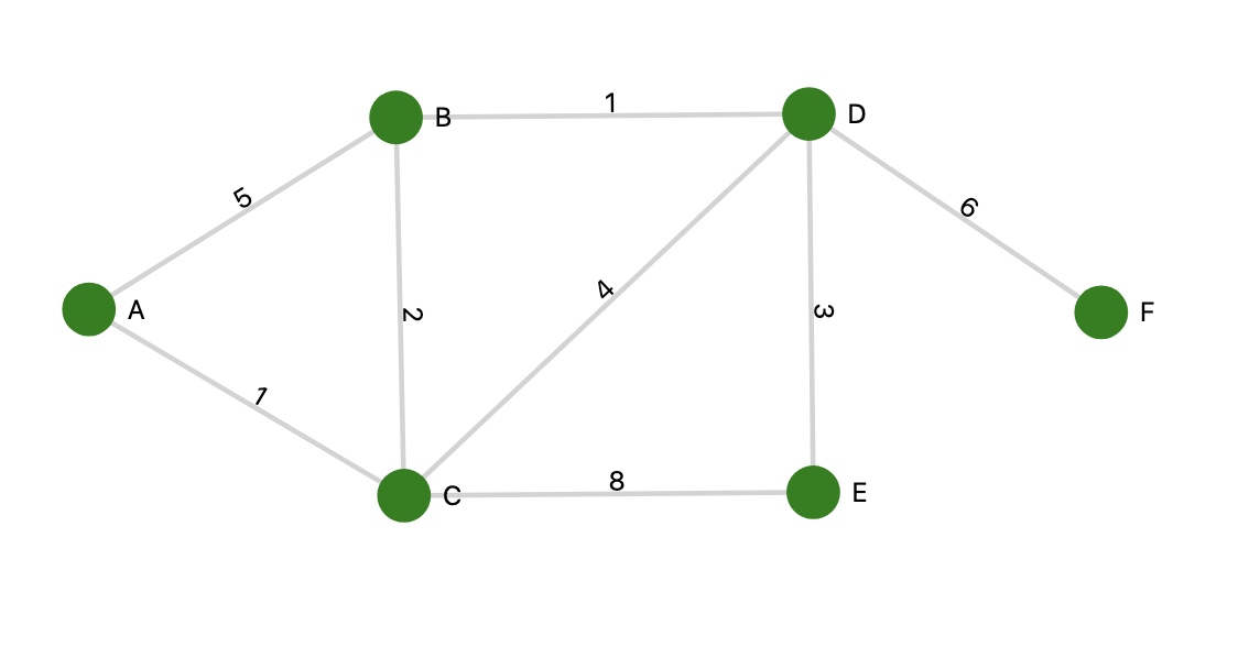
我们可以把该图的数据按照dict的格式导入到Python:
1 | graphs = { |
算法解析:
假设我们的起始点为A,pq展示的是heapq处理过的数据
1 | 1. 起始点A, pq=[{C, 1}(A-C), {B, 5}(A-B)], visited=[A], dist[A] = 0. 下一个node是C |
所以遍历的顺序为: [A,C,B,D,E,F](可以理解为[A,C,B,D,E] 和 [A,C,B,D,F])
具体代码实现:
1 | """ |
LinkList algorithm
首先定义一个List Node的class:
1 | class ListNode: |
常见问题
如何找到链表的中间元素?
可以采用快慢指针的原理,第一个指针向后走一步,第二个指针向后走两步,这样第二个指针结束的时候第一个指针刚好到中间
1
2
3
4
5
6
7
8
9
10
11
12
13
14def find_mid(head):
"""
找到该list中间的元素
:param head: the head of list
:return:
"""
slow = head
fast = head
while fast.next is not None and fast.next.next is not None:
slow = slow.next
fast = fast.next.next
return slow使用递归的思想来解决这个问题,在递归的时候我们已经可以得到相对应的长度,可以找到中点位置
1
2
3
4
5
6
7
8
9
10
11
12
13
14
15
16
17def find_mid_recursion(node, index):
"""
find the mid by recursion
:param node:
:param index:
:return:
"""
global mid
if node.next is not None:
find_mid_recursion(node.next, index+1)
else:
mid = int(index / 2)
if mid == index:
return node
return None判断链表是否有环
也可以通过使用快慢指针的思想来解决这个问题。当慢指针和快指针重合的时候代表着有环(但是容易进入死循环)。比如1->2->3->1,这样就是一个简单的环,当slow指向2的时候fast也指向2,所以表示有环
1
2
3
4
5
6
7
8
9
10
11
12
13
14
15
16
17def check_cycle(node):
"""
check whether exist cycle in the linklist
:param node:
:return:
"""
slow = node
fast = node
while fast.next is not None and fast.next.next is not None:
slow = slow.next
fast = fast.next.next
if slow == fast:
return True
return False反转链表
使用recursion来实现反表。
1
2
3
4
5
6
7
8
9
10
11
12def reverse_recursion(curr, next):
"""
reverse the link list by recursion
:param curr:
:param next:
:return:
"""
if next is None:
return
reverse_recursion(next, next.next)
next.next = curr
curr.next = None不用递归的实现方法。
1
2
3
4
5
6
7
8
9
10
11
12
13
14
15
16def reverse(node):
"""
reverse the link list without recursion
:param node:
:return:
"""
curr = node
next = node.next
curr.next = None
while next is not None:
temp = next.next
next.next = curr
curr = next
next = temp删除经过排序的链表中重复的节点。
判断当前数字是否和下一个相等,如果相等,记录该node,继续循环,找到与改数字不相同的数字,然后把curr.next = 该不相同node
1
2
3
4
5
6
7
8
9
10
11
12
13
14
15
16
17
18
def find_diff(node):
"""
in a sort link list, remove the duplicate value
:param node:
:return:
"""
curr = node
record = None
while curr.next is not None:
next_node = curr.next
if curr.val == next_node.val and record is None:
record = curr
elif curr.val != next_node.val and record is not None:
record.next = next_node
record = None
curr = curr.next计算两个链表数字之和
将链表代表的数字进行相加即可,注意首位代表的是个位。3->1->5 代表513,5->9->2 代表295,最终计算结果为 8->0->8, 808。
1
2
3
4
5
6
7
8
9
10
11
12
13
14
15
16
17
18
19
20
21
22
23
24
25
26
27
28
29
30
31
32
33
34
35def sum_list(l1, l2):
"""
add two link list together
将链表代表的数字进行相加即可,注意首位代表的是个位。3->1->5 代表513,5->9->2 代表295,最终计算结果为 8->0->8, 808。
:param l1:
:param l2:
:return:
"""
over_ten = False
s = ListNode(0)
head = s
while l1 is not None or l1 is not None:
v1 = l1.val if l1 is not None else 0
v2 = l2.val if l2 is not None else 0
sum_value = v1 + v2
sum_value = sum_value + 1 if over_ten else sum_value
if sum_value >= 10:
over_ten = True
sum_value = sum_value % 10
s.val = sum_value
l1 = l1.next if l1 is not None else None
l2 = l2.next if l2 is not None else None
if l1 is None and l2 is None:
break
else:
s.next = ListNode(0)
s = s.next
return head链表-奇数位升序偶数位降序-让链表变成升序
先拆分链表,然后把偶数链表翻转,然后合并
比如list为:1 10 2 9 3 8 4 7 5 6
奇数链表为:1 2 3 4 5
偶数链表为:10 9 8 7 6
1
2
3
4
5
6
7
8
9
10
11
12
13
14
15
16
17
18
19
20
21
22
23
24
25
26
27
28
29
30
31
32def merge_two_list(l):
"""
split to two list
:param l:
:return:
"""
odd = ListNode(0)
even = ListNode(0)
odd_head = odd
even_head = even
index = 1
while l is not None:
if index % 2 != 0:
odd.val = l.val
odd.next = ListNode(None)
odd = odd.next
else:
even.val = l.val
even.next = ListNode(None)
even = even.next
l = l.next
odd = None
even = None
reverse_recursion(odd_head, odd_head.next)
reverse_recursion(even_head, even_head.next)
# merge them together最后这个部分由于处理不太得当,所以写起来有点麻烦,先搁置一下
一个单向链表,删除倒数第N个数据。
首先准备两个指针,第一个指针先走n个,然后第二个出发,当第一个指针为None时,第二个指针刚好指向该数据
1
2
3
4
5
6
7
8
9
10
11
12
13
14
15
16
17
18def delete_n_element(l, n):
"""
删除倒数n的element
:param l:
:param n:
:return:
"""
index = 0
curr = l
corr = l
while curr is not None:
if index >= n + 1:
corr = corr.next
curr = curr.next
index += 1
print(corr.val)
KMP string match
Worst case: $O(m+n)$
Two stages:
- Pre-processing: table building O(m)
- Matching: O(n)
Space complexity: O(m)
*首先需要制作一个prefix table: *
这个是根据字符串的前后字符有一个相等的, i-len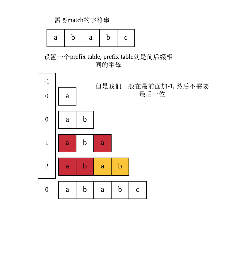
这样的话我们的prefix就制作好了-1,0,0,1,2.
然后我们需要根据这个table来进行KMP的search的算法: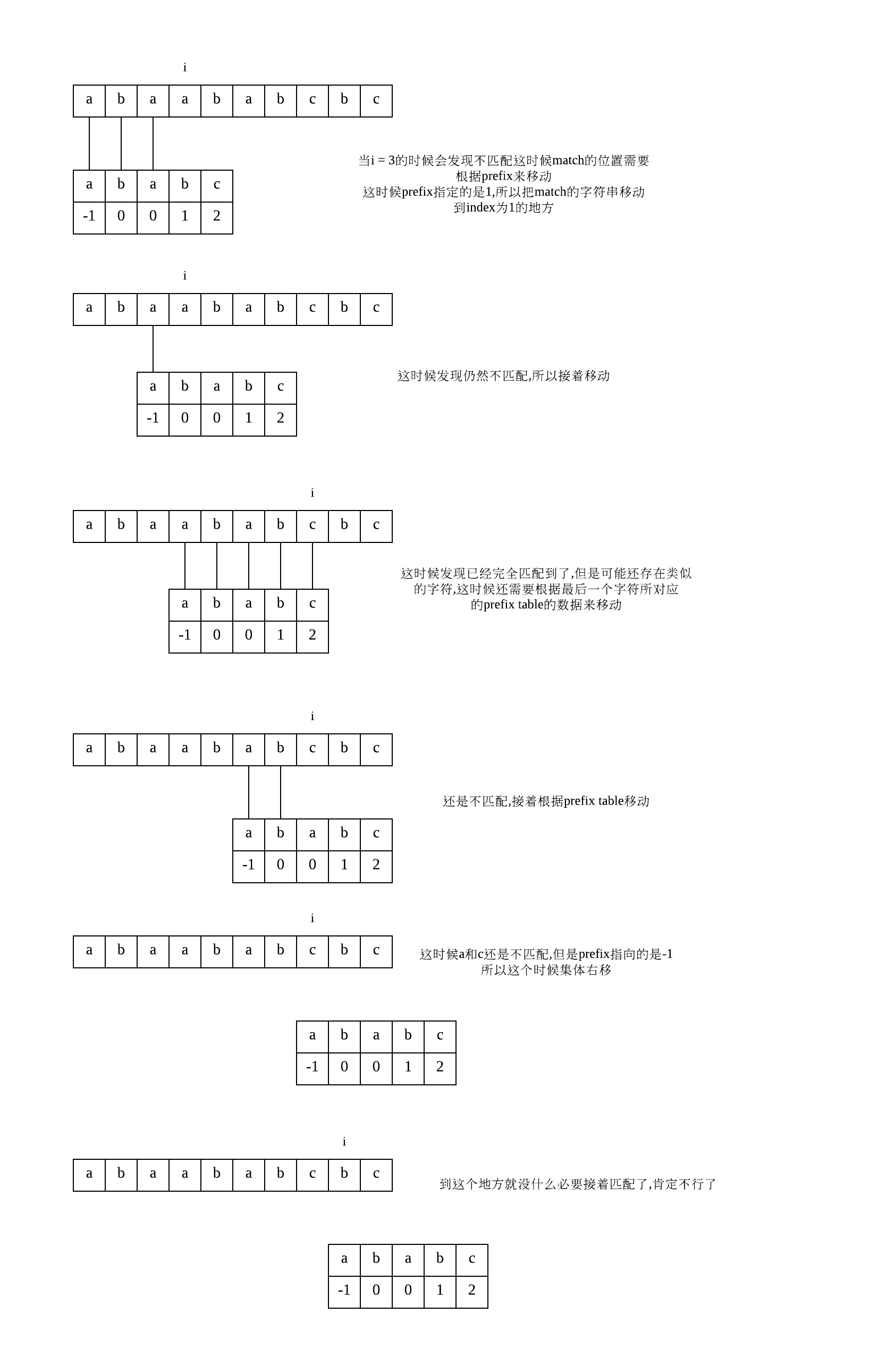
具体的实现代码:
1 | package KMP; |
录制了一个短视频来了解一下:
Tree
昨天顺便看了一下关于tree的一些常用算法,给大家看一下。
首先tree要有一个node:
1 | package tree; |
然后是对tree的一些常用操作的代码,都是使用递归来完成的:
1 | package tree; |
回溯算法
可以理解为一个决策树的遍历过程,我们只需要考虑:路径,选择列表,结束条件。 伪代码如下:
1 | result = [] |
核心在for里面的循环,递归之前调用make a select,递归之后drawback select
比如LeetCode里面的 *46. Permutations * 一个排列组合的问题:
1 | import java.util.ArrayList; |